8.4
CD++Modeler
Using
the CD++ Modeler Graphical User Interface (GUI), atomic and coupled models can
be created for the CD++ toolkit. The basic functions of the GUI include:
creating atomic and coupled models, exporting the models to different formats,
and animating the simulations. The GUI
also includes: - a simple text editor to directly modify Cell-DEVS models, -
the RUN/SIMU commands to execute the simulation with the CD++ toolkit, and -
the DRAWLOG command to generate the draw information from the simulation. This
section describes in detail how to use the GUI for inputting DEVS model, and
for visualizing the results of the Cell-DEVS, Atomic-DEVS, and Coupled-DEVS
models.
Since the GUI is coded in Java (JDK1.4.1[MSOffice1]), it is platform portable and can be run in various
environments, such as Eclipse or JBuilder (with JDK 1.4.1[MSOffice2]). Although this tool is a standalone program, it can also be accessed
through CD++Builder by clicking on ![]() ,
located in menus of CD++Builder, CELL-DEVS, DEVS, and GGAD perspectives.
,
located in menus of CD++Builder, CELL-DEVS, DEVS, and GGAD perspectives.
8.16.1 To install and run the standalone GUI:
Note: If you are using CD++Builder, you don’t have to install
the standalone version. You can access CD++ Modeler directly from the Cellae’s
perspective, by clicking on ![]() .
.
1) Download the cdModeler.zip file, which contains
source code, class files, and some example files. Decompress the cdModeler.zip file in the
Windows environment.
2) Install JDK 1.4.1[MSOffice3] or above.
3) Set
up the JAVA_HOME environment variable to point to the JDK directory.
To do this, modify the PATH environment variable by
adding " %JAVA_HOME%\bin; ".
Note: To modify environment variables, go to Control
Panel > System > Advanced > Environment Variables.
In the cdModeler directory, double click the run.bat
file to start the program.
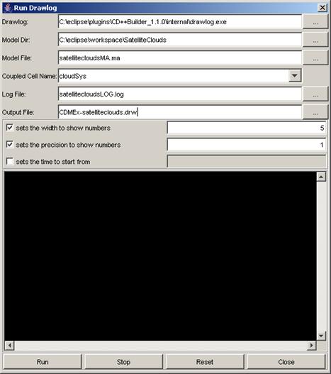
When the program has started, it will display a dialog as seen in Figure 127.
8.16.1.1 Using CD++Modeler
Once
the CD++Modeler tool is running, the following screen will appear.
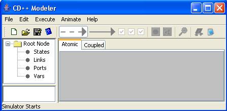
Figure 127: CD++ Modeler window.
![]()
Figure 128: CD++ Modeler menu bar.
![]()
1
2 3 4
5 6 7
8 9 10 11
12 13 14
Figure 129: CD++
Modeler button bar.
The button bar contains the
following buttons (in order from left to right):
- New - new
project
- Open - open project
- Save -
save current activity
- Help -
- Internal Link - only used for the
atomic model design space
- External Link - only used for the atomic
model design space
- Show Link Expressions - only used for the atomic model
design space
- Show Link Actions - only used for the atomic model
design space
- Show Link Ports - only used for the coupled
model design space
- Add new Atomic Model
Unit - only used for the coupled
model design space
- Add new Coupled Model
Unit - only used for the coupled
model design space
- Close Exploded Unit - only used for coupled model
design space
- Simulate - only used for coupled
mdoel design space
- Editor - Doesn’t work when modeler is exported as a JAR
Please see the Help files
(in Atomic>Distribution and Coupled>Distribution) for a more detailed
description of the button bar.
The following sections
explore the functions of the GUI with examples.
8.16.2 Creation of DEVS Models (using the design space)
Models can be defined within
the design space. First select the
appropriate design space (Atomic or Coupled) for the model by clicking on the
appropriate tab.
8.16.2.1
Create Atomic Model
The basic steps required for
creating an atomic model are as follows:
1) Choose the atomic design
space by clicking once on the Atomic tab in the interface.
(The atomic design space
consists of a central panel and two lateral panels.)
2) Select File > New from the main menubar.
3) Position the mouse within
the design space, and right-click. The
following popup menu will be displayed.
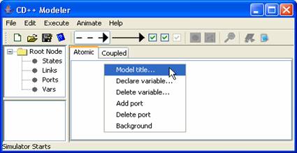
Figure 130: Creating an atomic
model
8.16.2.1.1 Setting the Model Title
1) Left-click on Model title. The Set Title ("Model ClassName") dialog will be displayed.
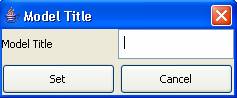
Figure 131: Entering the model title
2) Type in the appropriate
Model Title, and press Set.
8.16.2.1.2 Adding Units
1) Left double-click on the
design space. A circular unit will be drawn in blue.
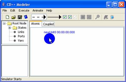
Figure 132: Adding Units to an Atomic Model
2) Left double-click on the
circular unit. This will select the circular unit, as represented by the unit
becoming red.
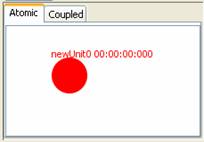
Figure 133: Selecting a unit
3) Left double-click on the
selected unit. This will de-select the circular unit, as represented by the
unit returning to blue.
8.16.2.1.3 Setting Properties of Units
4) Right-click on the circular unit. The following popup menu will be displayed.
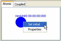
Figure 134: Setting initial property units
5) To set this unit as the initial unit of the model,
left-click on Set initial.
When
another unit is set as the initial unit of the model, the previous unit is
automatically de-selected as the initial unit.
6) To set the properties of this unit, left-click on
Properties. The State Properties
("Atomic Unit properties") dialog will be displayed. Type in the
appropriate state ID and state Time-to-Leave.
Press OK.
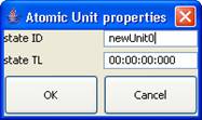
Figure 135: Entering State ID and state TL
8.16.2.1.4 Deleting Units
7) Select the circular unit (ie. left double-click on
the circular unit). After the unit
becomes red, press the Delete button on the keyboard, or select Edit>Delete from the main
menubar.
When a
unit is deleted, all links connected to the unit will also be deleted.
To delete multiple units, select the multiple units
(ie. left double-click on each of the units), and press Delete or Edit>Delete.
8.16.2.1.5 Adding Ports
1) Right-click within the "canvas" (design
space). The following popup menu will be
displayed.
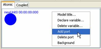
Figure 136: Adding ports
2) Left-click on Add
port. The
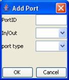
Figure 137: Entering Port ID
Repeat this procedure to add all the necessary ports
for a unit.
8.16.2.1.6 Deleting Ports
3) Right-click within the "canvas" (design
space). The following popup menu will be
displayed.
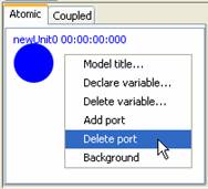
Figure 138: Deleting Ports
4) Left-click on Delete
port. The
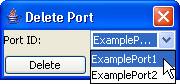
Figure 139:
8.16.2.1.7 Adding Links
Links represent transitions between different or
similar units. After creating all the necessary atomic units, links can be made
between the units or be created as a selflink.
Two types of links are available for atomic models:
Internal link (representing an internal transition):
Transition happens automatically as a timer runs out.
External link (representing an external transition):
Transition happens when a certain expression returns true.
Steps to creating a link:
1) Before drawing a link, the user should select the
desired link type by clicking either the internal or external link button on
the toolbar.
2) To
draw a link between two units, position the mouse on one of the units, press
and hold the left mouse button on one unit, drag the mouse to the other unit,
and release the left mouse button. A link with the pre-selected type will be
drawn.
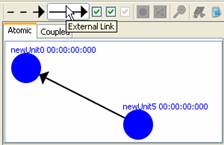
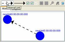
Figure 140: Adding links (external and internal)
3) To create a 'self link'
(a link between an atomic unit and itself), position the mouse cursor on the
unit. Make shure that the unit is not selected [unit is not coloured in red].
Press and hold the left mouse button. Drag the mouse away from and back to the
unit with the left mouse button being held. Release the left mouse button to
finish creating the self link.
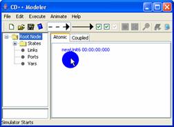
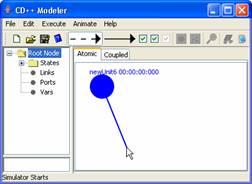
Figure 141: Creating a self link
A Warning Message dialog
will be displayed, verifying the creation of a self link. Click OK.
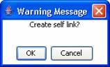
Figure 142: Warning message for creating a self link
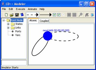
Figure 143: Example of internal and external
selflinks attatched to an atomic unit
8.16.2.1.8 Adding Transition Events to Internal and External Links
Internal Link Transition: To attach a port and value assignment to an internal
link, right-click on the link. The following popup menu will be displayed.
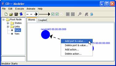
Figure 144: Attaching a link to a port
Left-click on Add
port & value. The Add port & value dialog box will be displayed
(See Figure 145). Select the appropriate port [output ports are for
internal transition], and type in the appropriate value for the port. Press OK.
When an internal transition occurs the selected output port will receive
the assigned value which is set in the Add port & value dialog box.
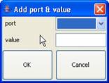
Figure 145: Adding port and value dialog box
External Link Transition: These transitions will allow transitions between
different atomic units [states]. In general the transition happens when a
user-defined value is received on a specific input port.
To add an expression to an external link [represented
by a solid arrow] the following must be done:
1)
Right click on
the on the external link. And select Edit
Expression....
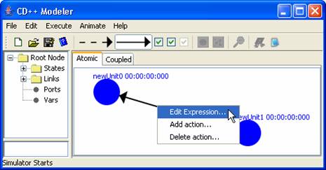
Figure 146: Adding an
expression to an external link
2)
Expressions can
be either added manually [if you know what to type] or with the help of the Add Function button. Inorder to use the Add Function button first select a
function to add from the bottom text field then click on the Add Function button. Now a dialog box
will pop up asking for parameters required in the function. Fill in the
parameters and click ok. Now that a
function is added, user must MANUALLY configure the rest of the expression by
typing “?value” [without the quotes] after the expression. The “value”
represents any number. An example external transition expression would be:
Value(in)?2 . This simply means that when the value at the port “in”
[represented by the Value(port) function] is equal to “2” then make a
transition to the other state.
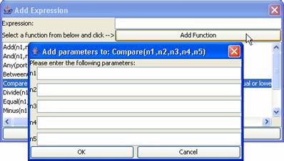
Figure 147: Showing a
dialog window when the Add Function button is clicked.
8.16.2.1.9 Deleting Links
5) Select the link (ie. left double-click on the
link). After the link becomes red, press
the Delete button on the keyboard, or select Edit>Delete from the main menubar.
To
delete multiple links, select the multiple links (ie. left double-click on each
of the links), and press Delete or Edit>Delete.
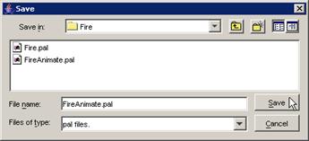
8.16.2.1.10 Saving and exporting the model
1) To save the model to disk, select File>Save or File>Save As from the
main menubar. The model will be saved as
a .gam file.
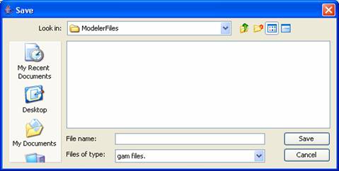
Figure 148: Save file Dialog box
2) In order to use the model in the[MSOffice4] other CD++ tools, the model must be exported to a
standard .cdd file. To export the model,
select File>Export. *.cdd must be the file name extension.

Figure 149: Choosing cdd files only
3) To save and export the model in one step, select
File>Save and Export.
8.16.2.2 Create Coupled Model
The basic steps required for creating a coupled model
are similar to those for creating an atomic model.
Open CD++ Modeler and choose the coupled design space
by clicking once on the Coupled tab in the interface.
The coupled design space consists of a central panel
and three lateral panels:
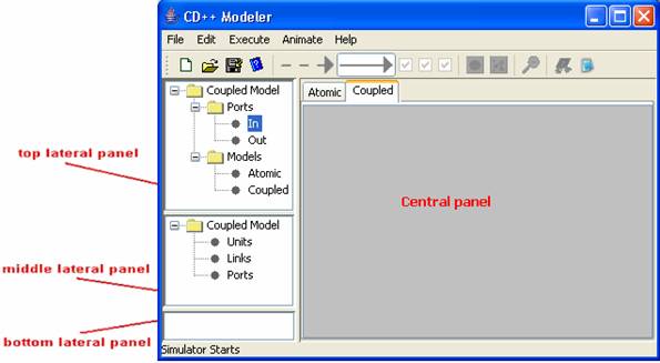
Figure 150: The coupled design space
The central panel displays the objects (in graphical
form) of the coupled model. Objects
(such as ports, atomic models, and coupled models) can be added, and links can
be connected between the objects.
The top lateral panel displays the types of objects
that are available for defining the model. It is divided into ports (input and
output), predefined atomic models, and predefined coupled models.
The middle lateral panel displays the objects (in
textual form) that define the model.
(The textual form of the objects in the middle lateral panel correspond
to the graphical form of the objects in the central panel.)
When an object/element is selected in the middle
lateral panel, the description/details of the element will be displayed in the
bottom lateral panel. (ie. The bottom lateral panel displays a description of
the element currently selected in the middle lateral panel.)
The central panel is referred to as the 'Modeling
Panel'.
The middle lateral panel is
referred to as the 'Units Panel/Tree'.
8.16.2.2.1 Adding Atomic Units
1) To add a new atomic model
that is not yet defined, click once on the Add
new Atomic Model Unit button. The new atomic model unit will be drawn in
the upper-left corner of the Modeling Panel, and will be given a default name
(eg. newAtomicModel0).
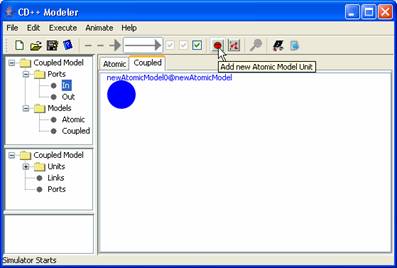
Figure 151: Adding atomic units
2) To edit the atomic model
unit, right-click on the unit. The following popup menu will be displayed.
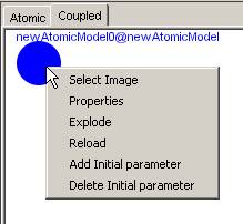
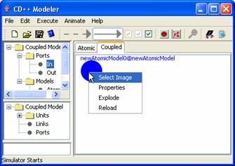
Figure 152: Right clicking on the image to edit
Select
Image - change the icon for the unit
Properties
- change the unit name
Explode
- explode the unit for its definition
Reload
- reload the unit if its
definition has been modified
3)
To change the unit name, left-click on Properties. The Model Properties dialog
will be displayed. Type in the appropriate Unit ID. Press OK.
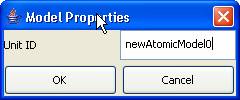
Figure 153: Changing unit name
The
Explode and Reload options will be described in later sections.
Adding
Coupled Models
1)
To add a new coupled model that is not yet defined, click once on the Add new
Coupled Model Unit button. The new coupled model unit will be drawn in the
upper-left corner of the Modelling Panel, and will be given a default name (eg.
newCoupledModel2).
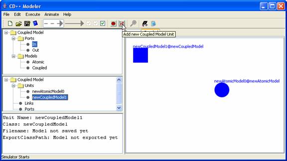
Figure 154: Adding coupled models
2) To edit the coupled model unit, right-click
on the unit. The following popup menu will be displayed.
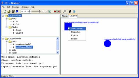
Figure 155: Editing a coupled model
Select Image - change the icon for the unit
Properties - change the unit name
Explode
- explode the unit for its definition
Reload
- reload the unit if its
definition has been modified
3)
To change the unit name, left-click on Properties.
The Model Properties dialog will be displayed. Type in the appropriate Unit
ID. Press OK.
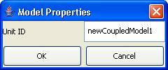
Figure 156: Changing the unit name
The
Explode and Reload options will be described in later sections
8.16.2.2.3 Adding Ports
Two types of ports are
available for coupled models: Input and Output.
1) To add a port, first select
the type of port in the top lateral panel. Within the canvas (design space),
position the mouse cursor at the desired location of the port. Left
double-click. The selected port type will be drawn, and will be given a default
name. For example, Port0 represents an
input port, while Port1 represents an output port.
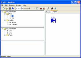
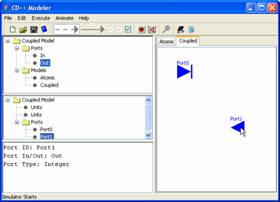
Figure 157: Adding ports
The
name of the port can be changed in two ways:
2a)
Right-click on the appropriate port. The following popup menu will be displayed.
Left-click on Properties.
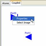
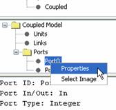
Figure158:
Changing the name of the port
2b)
In the Units Tree (the middle lateral panel), expand the Ports folder. Left
double-click on the appropriate port. An alternative method is to right click
on the appropriate port and select properties as seen in Figure158.
3)
The Port Properties dialog will be displayed. Type in the appropriate PortID.
Press OK.
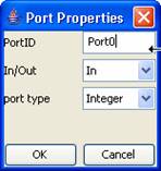
Figure 159: Entering port ID
Adding
Links
To add a link between two
objects, position the mouse cursor on the first object (the origin of the
link). Press and hold the left mouse button. Drag the mouse to the second
object (the destination of the link). Release the left mouse button. The link
will be drawn form the origin to the destination. For example, the origin of
the link is Port 2, while the destination of the link is newAtomicModel0.
The link will be created
only if both the origin and destination are valid.
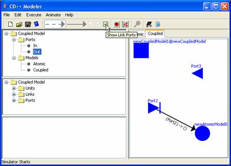
Figure 160: Adding links
NOTE: If you uncheck the Show link port checkbox then (Port2)->0 will not be displayed.
Selflinks can also be created for coupled models. One can add selflinks to the
coupled or atomic model unit as seen in Figure 161. Selflinks are added in the same way as one would add
a selflink to an atomic model (See section 8.16.2.1.7).
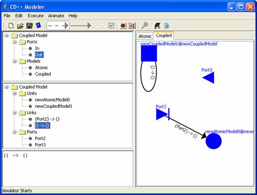
Figure 161:
Example selflink starts and ends at newCoupledModel1
8.16.2.2.5 Importing Models
A coupled model is composed of other atomic and
coupled models, which can be imported as predefined models. Three model types
are valid for importing:
-
predefined coupled models (.ma)
-
predefined atomic models (.cdd)
- basic
atomic models (from register.cpp)
For example, let’s consider
the ATM model.
You can download the
necessary files for the ATM model here: http://chat.carleton.ca/~jcao/blog/cd++files/ATM%20MODEL%20USING%20NEW%20CD%20MODELER.zip
Continue reading once you
have extracted the zip files.
Open CDModeler, click on the
coupled tab, click File>New to
start the creation of a new coupled model.
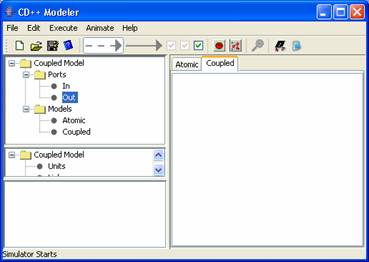
Figure 162: Fresh new coupled design space.
A predefined model can be
imported by selecting File>Import.
The Import dialog will be displayed. (Only .ma, .cdd, and .cpp files can be
imported.)
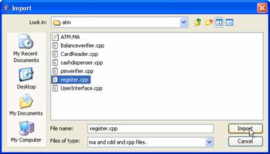
Figure 163: Import dialog box
Browse to the extracted
folder containing ATM files, select register.cpp,
and press Import. Now, a dialog box
will popup as a reminder that one must create ports to the model(s) before
adding them to the design space. Click OK.
In the top lateral panel
browse to Models>Atomic. The
CDmodeler window should now look like the following:
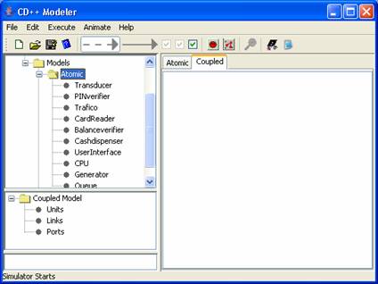
Figure 164: Showing imported models.
The name of the imported models will be displayed in
the top lateral panel, within the appropriate folder (Atomic or Coupled). In
this example the Register.cpp corresponds to a series of atomic models and thus
expanding the atomic subfolder one can find all the models associated with
Register.cpp.
For example: When a coupled model definition file
(.ma) is imported, the name of the imported model is displayed in the top
lateral panel under Models>Coupled. When an atomic model definition file
(.cdd) is imported, the name of the imported model is displayed in the top
lateral panel under Models>Atomic.
To add a unit of the imported model to the definition
of the current coupled model, first select the imported model name
(PINverifier) in the top lateral panel. Within the canvas (design space), at
the desired location of the unit, left double-click. A unit of the imported
model will be drawn.
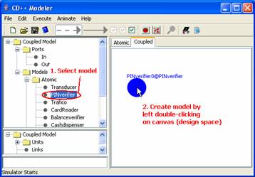
Figure 165: Creating a model on the canvas (design
space)
NOTE: Units of imported
models cannot be modified.
Importing an *.ma file:
Continuing from the previous
example, click File>Import. Browse
to the ATM folder again but this time select atmNEW.ma and click on import.
A coupled model definition
file (.ma) named "ATM" is imported:
(1) The name "ATM[MSOffice6]" is displayed in the top lateral panel under
Models>Coupled.
(2) “ATM9[MSOffice7]” (a unit of "ATM") is added to the
definition of the current coupled model [This is done by selecting ATM in the
top lateral panel and double clicking on the canvas (design space)].
(3) The predefined ports of “ATM9[MSOffice8]” are displayed in the middle lateral panel. (For "ATM", there are two output
ports: 'cash_out' and 'card_out'. There is also one input port: ‘in’.)
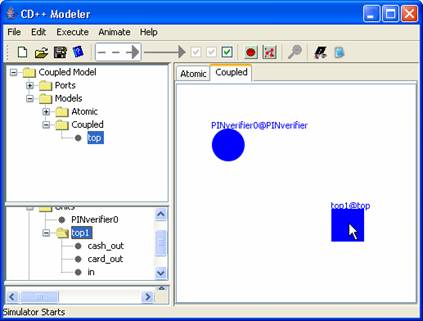
Figure 166: Importing and
creating a coupled model.
NOTE: Importing a *.cdd file undergoes the same
process as importing a *.cpp file the only difference is that one will need to
select a *.cdd file and the model imported will still be found in the Atomic subfolder.
Adding
ports to imported atomic models:
Ports can be added to any unit of the imported atomic
models.
To do so, follow the steps:
- Open CDModeler
- Click on the Coupled
tab
- Cick on File>New
- Import Register.cpp
- Expand the Atomic Subfolder by clicking on the
‘+’ beside the Atomic folder
- Left click to select the model one wishes to add
ports to. In this case select “Transducer”.
- Right click on “Transducer” and select Add port from the popup menu to add a port to “Transducer”.
(See Figure
167)
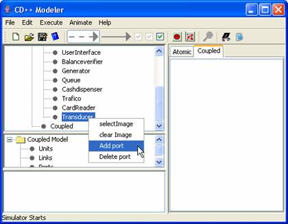
Figure 167: Adding a
port to imported model.
8.16.2.2.6 Exploding Models
A coupled model
(henceforth referred to as "current coupled model") is composed of
other atomic and coupled models (henceforth referred to as "component
models"), which (as demonstrated in previous sections) can be added as
blank models from the button bar or imported as predefined models.
These component
models (within the current coupled model) can be inspected, or
"exploded", for the purposes of definition and modification.
1) To explode a
component model, right-click on the model. The following popup menu will be
displayed. Left-click on Explode. A new model editor (henceforth referred to as
"exploded editor") will be displayed, in which the exploded model can
be edited. (The original model editor will be temporarily hidden, and will become
visible again after the exploded editor has been closed.)
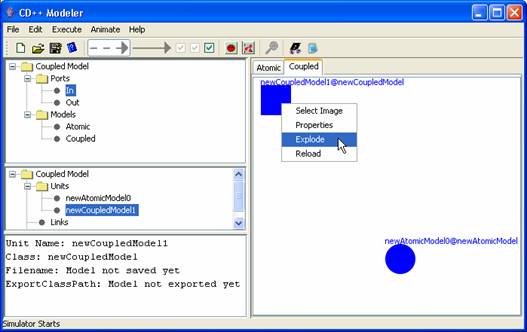
Figure 168: Explode model menu
If an atomic model is exploded, an atomic model
editor will be displayed. If a coupled model is exploded, a coupled model
editor will be displayed.
![[SCM]actwin,524,226,957,566;CD++ Modeler
java.exe
7/18/2006 , 10:49:00 AM](CDModeller_from_main_manual_files/image097.gif)
![[SCM]actwin,524,226,957,566;CD++ Modeler
java.exe
7/18/2006 , 10:48:19 AM](CDModeller_from_main_manual_files/image099.gif)
Figure 169: Atomic and Coupled editor corresponding to exploded
model
Note that within the exploded editor, the exploded
model type (ie. atomic or coupled) cannot be changed.
2) The exploded model can be edited using the same procedures as for
non-exploded models.
For example,
consider the following exploded coupled model, which was created for
newCoupledModel1 (seen in step 1).
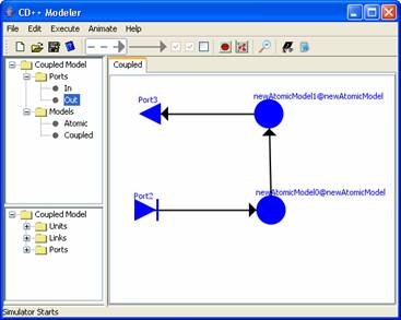
Figure 170: Editing exploded models
3) When the definition/modification of the exploded
model is complete one must close the exploded model and choose to save/cancel
the changes made in order to return to the original model editor.
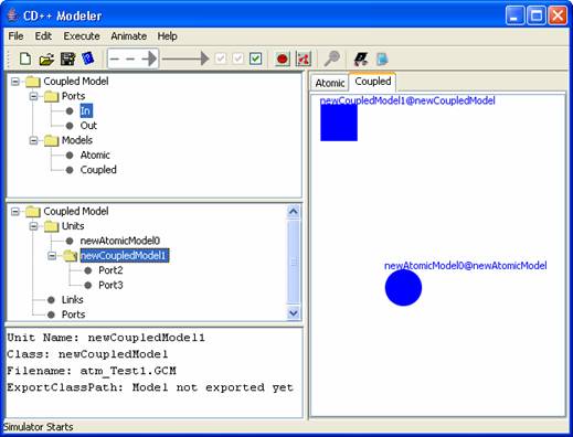
Figure 171:
Original Model Editor
The ports from
the exploded model (shown in step 2) are now available in the original model
editor (after saving). For example, the ports for newCoupledModel1 (ie. input
Port2 and output Port3) are displayed in the middle lateral panel, under
Coupled Model>Units>newCoupledModel1 (See Figure 171).
4) Once all
remaining component models are defined, links can be added between the ports of
the component models.
For example, once
newAtomicModel0 has been exploded and defined/modified, the ports for newAtomicModel0
(ie. input portA and PortB, and output PortC) will be displayed in the middle
lateral panel, under CoupledModel>Units>newAtomicModel0.
Additional ports
(ie. input Port3 and output Port4) can be added to the current coupled model,
and will be displayed in the middle lateral panel, under CoupledModel>Ports.
Links can be
added between the ports of the current coupled model and the ports of the
component models. These links will be displayed in the middle lateral panel,
under CoupledModel>Links.
In the current coupled model seen below, there are
three links:
(1) output PortC of newAtomicModel0 is connected to
input Port2 of newCoupledModel1
(2) input Port3 of the current coupled model is
connected to input Port2 of newCoupledModel1
(3) output Port3 of newCoupledModel1 is connected to
output Port4 of the current coupled model
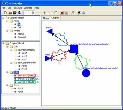
Figure 172: Coupled model with links
5) If a component
model is exploded for modification after links have been connected, the links
connected to the ports of the component model will be disengaged. This will
prevent unpredictable changes from occurring.
For
example, if newCoupledModel1 is exploded, the links connected to the ports of
newCoupledModel1 (i.e. input Port2 and output Port3) will be disengaged.
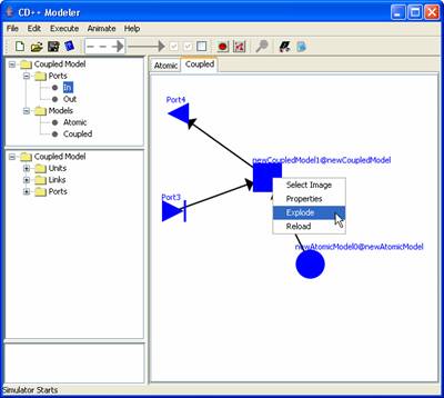
Figure 173: Disengaged
links on an exploded coupled model
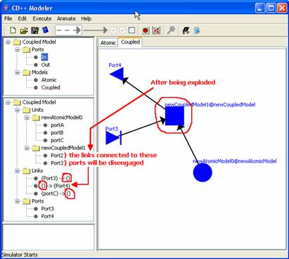
Figure 174: Detailed visualization of disengaged links
8.16.2.3 Adding Images to Models
Images can be added to a model in two ways.
One way is to set an image as a background, the second way is to set an image
to represent a unit within the model.
8.16.2.3.1 Adding Background
To add a background to the canvas; right
click on the canvas [white space] and select background (see Figure 175). When the
file browser window pops up select an image file to load and click Set.
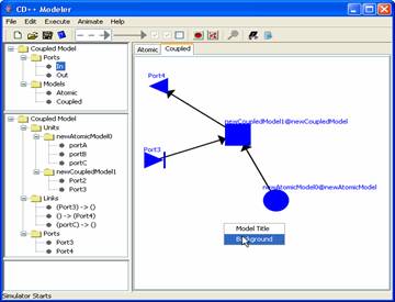
Figure 175: Loading
Background
Note: The menu you get when right clicking on the canvas may be
different than the one shown in Figure 175. This is because you are adding the background to the
atomic canvas and not the coupled canvas. However, the steps to add the image
is all the same. [Hint: click on Background]
Alter an image has been set as background you
should see the background image stretched to cover the whole canvas. (See Figure 176)
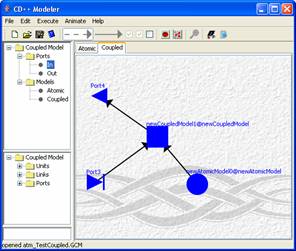
Figure 176: Image of a
car set as background
8.16.2.3.2 Adding Image to Units on Coupled Canvas
Note: Images can only be added to units [any object that is not a
link] on the coupled canvas.
Images can be added to atomic units, coupled units, input ports and
output ports.
To add an image right click on the unit and click Select Image (see Figure 177).
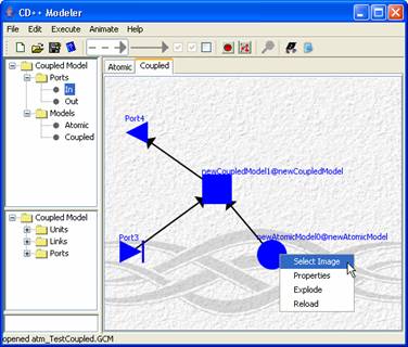
Figure 177: Adding image to unit
In the the file browser window select an image you wish to set as the
image for the unit and click Set.
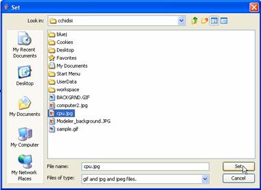
Figure 178: Choosing an image
The following is an example of having an image representing a unit
[note the yellow car].
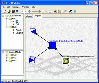
Figure 179: Image added to atomic unit
8.16.3 Visualization of DEVS models (using the Animate menu commands)
This section describes how to visualize the result
files of atomic Cell-DEVS models, atomic-DEVS models, and coupled-DEVS
models.
8.16.3.2 Model type selection
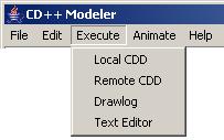
From the main menubar,
left-click on Animate. The following menu will be displayed. Select the
appropriate option, depending on the model type to be visualized:
Cell-DEVS animation -
atomic Cell-DEVS models
AtomicAnimate -
atomic-DEVS models
CoupledAnimate -
coupled-DEVS models
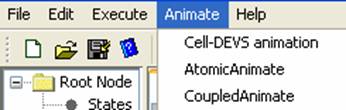
Figure 180: Animate menu
The following sections
describe the commands of the Animate menu for the version of CD++ Modeler
included in the CD++ Builder plugin for Eclipse, not the stand-alone version of
CD++ Modeler.
AtomicAnimate
using: Atomic-DEVS, Coupled-DEVS, Atomic Cell-DEVS
A DEVS model must include at least one atomic model.
After simulating the DEVS model, a .log file is generated. The .log file
records all the messages sent between DEVS components. This includes all messages sent/received by all atomic models
in the coupled model. The message values sent/received by a specific atomic
model can be extracted from the .log file and visualized.
The steps required for visualizing the message values
sent/received by a specific atomic model are as follows:
1) In the Animate menu, left-click on AtomicAnimate.
An atomic animate dialog box will be displayed.
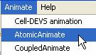
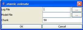
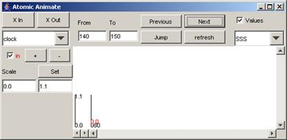
Figure 181: Atomic Aniamte Options
2) Left-click on the browse button[MSOffice9]. A Set dialog will be displayed. Select the .log
file that contains the messages sent/received by the atomic-DEVS model to be
visualized. (The atomic-DEVS models that send/receive messages within the
selected .log file will be available for visualization.) After choosing the
appropriate .log file, left-click on Set.
![[SCM]actwin,430,394,780,524;Set
java.exe
7/20/2006 , 11:04:42 AM](CDModeller_from_main_manual_files/image127.gif)
Figure 182: Set dialog box
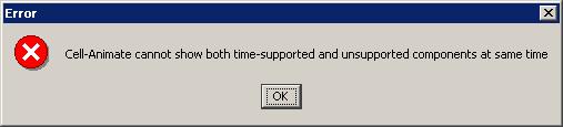
If an [MSOffice10]invalid file type is chosen, the (blank) visualization window
will be displayed as follows:
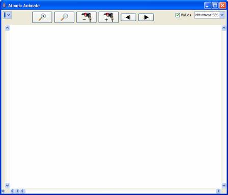
Figure 183: Empty visualization window due to invalid file type
The following example demonstrates the functionality
of the Atomic Animate visualization window, using the atomic-DEVS model
FunctionEval (which was extracted from the Hybrid model). Additional examples for a coupled-DEVS model
(4BitCounter) follows.
AtomicAnimate
Example of Atomic-DEVS: FunctionEval
To run this example, download the FunctionEval
project. Where
would one download this?
FunctionEval is an atomic-DEVS model that contains
one output signal.
In the Set and atomic animate dialogs, open
tester_caso1.log.
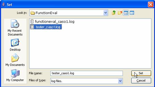
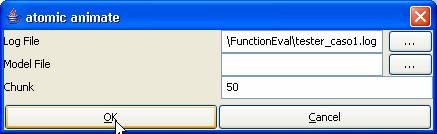
Figure 184: Opening tester_caso1.log
The atomic-DEVS models that send/receive messages
within tester_caso1.log will be available for visualization. Since
tester_caso1.log only contains the messages sent/received by the
function@FunctionEvaluator model, the only atomic-DEVS model available for this
example is the function model.
The following Atomic Animate visualization window
will be displayed.
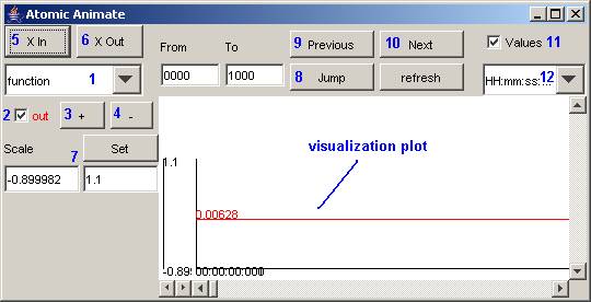
Figure 185: Atomic Animate visualization window
The Atomic Animate visualization window has several
functions for modifying the appearance of the visualization, such as:
-select
the atomic-DEVS model to be visualized (1)
-select
the output signals (of the selected atomic-DEVS model) to be plotted (2)
-zoom
in/out on the vertical axis (3, 4) and the horizontal axis
(5, 6) of the plot
-set the
upper and lower bounds of the vertical scale (7)
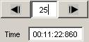
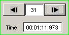
-jump to
the specified time interval (8)
-go to
the previous/next time interval (9, 10)
-show the
values of the output signal on the plot (11)
-select
the time format to be displayed on horizontal axis (12)
Select the atomic-DEVS model to be visualized
1) Left-click on the drop-down list. From the
drop-down list, select or left-click the atomic-DEVS model to be visualized.
The output signals of the selected atomic-DEVS model will be displayed.
In this example, the only atomic-DEVS model available
for visualization is the function model.
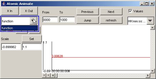
Figure 186:Atomic DEVS model visualization
8.16.3.4.2 Select the output signals to be plotted
1) To remove a signal from the visualization, uncheck
or left-click the box beside the signal name. The plot of the output signal
will be removed from the visualization window.
In this example, the function model has one signal, out.
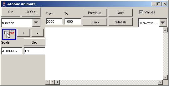
Figure 187: Removing output signal from visualization window
2) To include a signal in the visualization, check or
left-click the box beside the signal name.
8.16.3.4.3 Select the time format for the horizontal axis
1)
Left-click on the drop-down list located below the Values checkbox. From the drop-down list, select or left-click
the appropriate time format to be displayed on the horizontal axis.
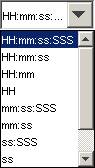
HH - represents hours
mm - represents minutes
ss - represents seconds
SSS - represents milliseconds
Figure 188: Values drop down menu
In this example, the time selected time format is SSS
(which represents milliseconds).
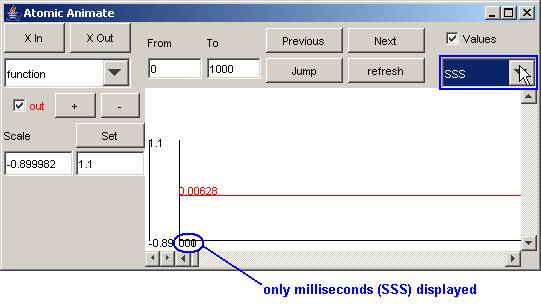
Figure 189: Specifying time
The entire visualization plot for the out signal of function model appears as follows:
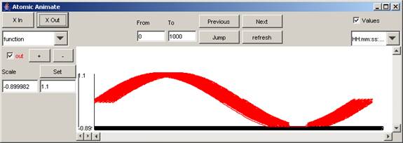
Figure 190: Visualization of the out signal
For upcoming sections, the following plot will be
modified:
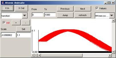
Figure 191: Plot to be modified
8.16.3.4.4 Show the values of the output signal on the plot
1)
To remove the output signal values from the plot, uncheck or left-click the box
beside Values. The values of the output signal(s) will be removed from the
visualization.
In this example, the values of the signal out are removed, and so are
no longer visible.
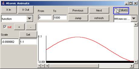
Figure 192: Removing values of the out signal
2) To include the output signal values in
the plot, check or left-click the box beside Values. The values of the output signal(s) will be
added to the visualization.
In this example, the values of the signal
out are added, and so are visible. (The
values are not legible due to their proximity.)
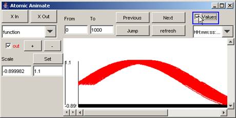
Figure 193: Adding the values of the out signal (making the
signal visible)
Note: When the plot is zoomed in (and the
time format changed), the values can be made legible:
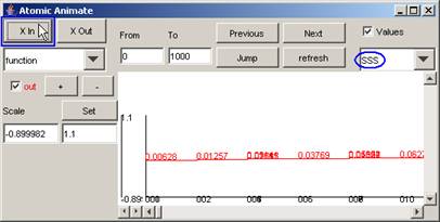
Figure 194: Viewing the values only
(Zooming in and out of the horizontal
axis is described in the following section.)
Zoom
in or out of the horizontal axis of the plot
1) To 'zoom in' or stretch the horizontal scale,
press the X In button. The length of the horizontal scale will increase.
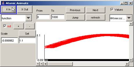
Figure 195: Zooming in on the horizontal scale
2) To 'zoom out' or compress the horizontal scale,
press the X Out button. The length of the horizontal scale will decrease.
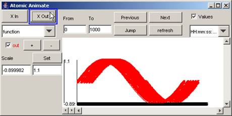
Figure 196: Zooming out on the horizontal scale
Zoom
in or out of the vertical axis of the plot
1) To 'zoom in' or stretch the vertical scale, press
the + button. The length of the vertical scale will increase.
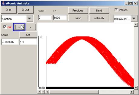
Figure 197: Zooming in on the vertical scale
2) To 'zoom out' or compress the vertical scale,
press the - button. The length of the vertical scale will decrease.
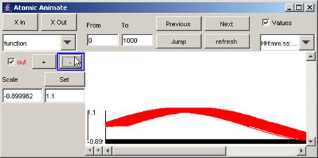
Figure 198: Zooming out on the vertical scale
8.16.3.4.7 Set the lower and upper bounds of the vertical scale
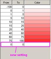
1) To set the lower and upper bounds of the vertical
scale, first specify the desired lower and upper bounds in the Scale fields.
In this example, the upper bound is specified as 2.0,
while the lower bound remains unchanged.
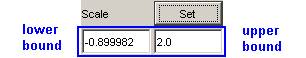
Figure 199: Setting lower and Upper bounds
2) Press the Set button. The parts of the output
signal that fall within the lower and upper bounds will be displayed. (The
values for the lower and upper bounds are visible on the vertical axis.)
In this example, the parts of the output signal that
fall within -0.899982 and 2.0 on the vertical scale are displayed.
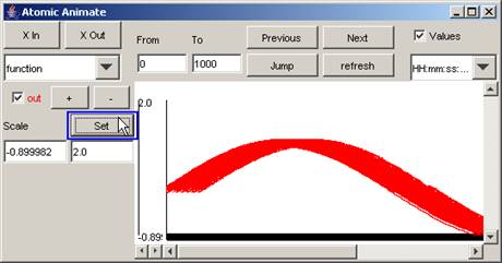
Figure 200: Displaying the signal between the lower and upper
bounds
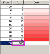
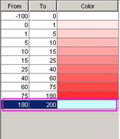
8.16.3.4.8 Jump to the specified time interval
1) To go directly to a particular time interval of
the visualization, first specify the desired range of the time interval in the
From and To fields.
In this example, the To field (or upper bound of the
time interval range) is specified as 100, while the From field (or lower bound
of the time interval range) remains unchanged.
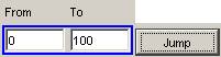
Figure 201:Specifying desired range of time
2) Press the Jump button. The parts of the output
signal that occur at times that fall within the From and To range will be
displayed. (The values for the time interval range are visible on the
horizontal axis.)
In this example, the parts of the output signal that
occur between 0 and 100 (milliseconds) are displayed.
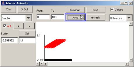
Figure 202: Viewing only the specified time range
Note: When zoomed in (ie. by pressing the X In button
several times), the plot from the previous figure will appear as follows:
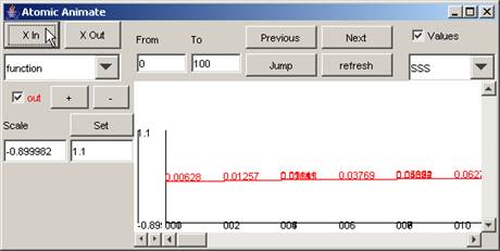
Figure 203: Zooming in to the previous plot
Go
to the previous/next time interval
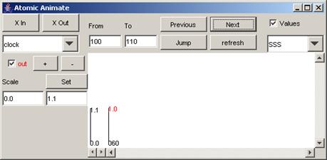
1) To go to the next increment of the specified
interval, press the Next button.
In this example, using the same time interval as
previously specified, when the Next button is pressed, the parts of the output
signal that occur between 100 and 200 (milliseconds) are displayed.
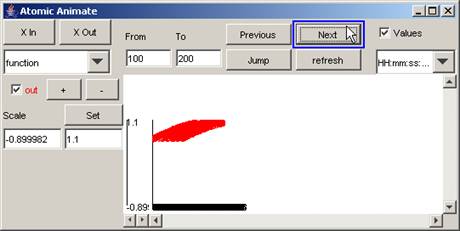
Figure 204: Going to the next time interval
In this example, when the Next button is pressed
again, the parts of the output signal that occur between 200 and 300
(milliseconds) are displayed.
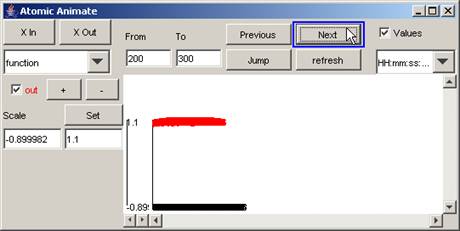
Figure 205: Signal between 200 and 300 milliseconds
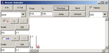
2) To go to the
previous increment of the specified interval, press the Previous button.
In this example,
when the Previous button is pressed, the parts of the output signal that occur
between 100 and 200 (milliseconds) are displayed. This is the same plot as the first plot seen
in step 1.
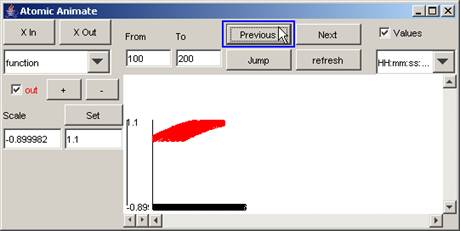
Figure 206: Going to the previous increment
Jump
to a specific time
1) To go directly to a specific instance
of time of the visualization, first specify the instance in both the From and
To fields.
In this example, the specific instance to
be plotted is 200.
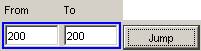
Figure 207: Jumping to a specific instance
2) Press the Jump
button. The part of the output signal that occurs at the specified instance
will be displayed. The value for the specified instance of time will be visible
on the horizontal axis. The output value for the signal at the specified
instance will be visible on the plot.
In this example,
the part of the output signal that occurs at the instance of 200 (with a
corresponding time of 196 milliseconds) is displayed. The output value of the
signal at 196 milliseconds is 0.94299.
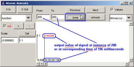
Figure 208: Viewing a specific instance
Note: When the From and To fields contain the same value,
the Previous and Next buttons are inoperable.
Note: As demonstrated earlier, when output
signal values are removed from the plot (by unchecking the Values checkbox), no
output values will be displayed. A red line representing the range of values of
the output signal will be visible.
In
this example, when the single output signal value is removed from the plot, the
red line is barely visible, since the "range" of the output signal is
limited to one single value.
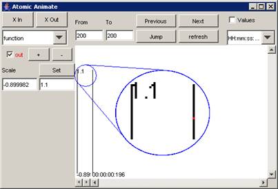
Figure 209
: Range of output signal limited to one value
AtomicAnimate
Example of Coupled-DEVS: 4BitCounter
To run this
example, download the 4BitCounter project.
4BitCounter
is a coupled-DEVS model composed of multiple atomic-DEVS models that each
contain multiple output signals.
The
main functionality of the Atomic Animate visualization window described in the
previous example (FunctionEval) also applies for this example. However, while
the previous example (FunctionEval) illustrated the visualization of a single
atomic-DEVS model, this example (4BitCounter) illustrates the visualization of
(a coupled-DEVS model composed of) multiple atomic-DEVS models.
Using the same
procedure as in the previous example, in the Set and atomic animate dialogs,
open 4Counter.log.
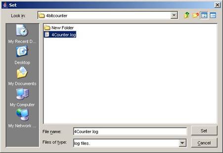
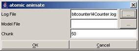
Figure 210: Opening 4Counter.log
The models that
send/receive messages within 4Counter.log will be available for visualization.
The file 4Counter.log contains the messages sent/received by the top model,
which is composed of the following models: 4count@Process_4_Counter,
b1@Signal, b2@Signal, b3@Signal, b4@Signal, clock. Whereas the first four models are atomic-DEVS
models, the fifth model, clock, is a coupled-DEVS model composed of the
atomic-DEVS models: inv@Process_Inv, sig1@Signal. So, for this example, the following models/components
are available for visualization: clock, 4count, inv, b4, b3, top, b2, b1, sig1.
The following Atomic Animate visualization window
will be displayed.
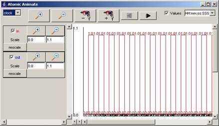
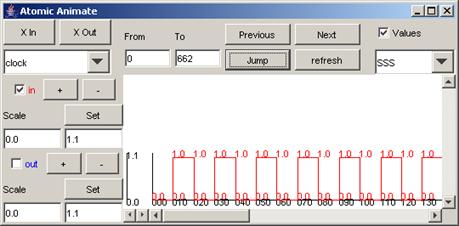
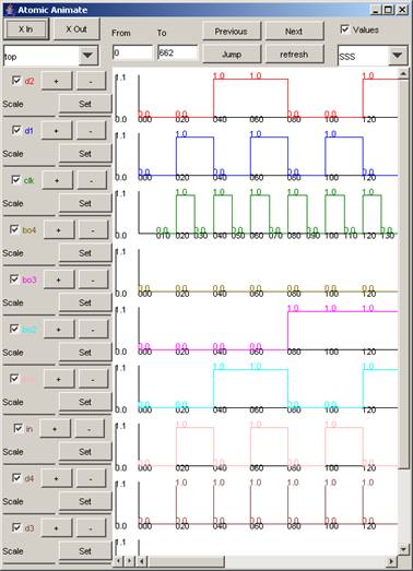
Figure 211: Atomic Animate Visualization Window
By default, the
signals of the first model/component in the list - in this example, clock -
will be displayed.
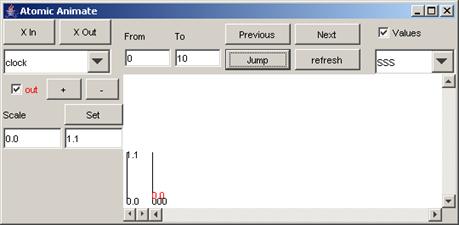
Also by default
the visualization plot will display the range of output values of the selected
signals for the time interval spanning the entire simulation. In this example,
the time interval of [
Also
by default, the lower/upper bounds of the vertical Scale will initially
correspond to the minimum/maximum of the output value range. So, the vertical
scale for an output signal will automatically be set such that the entire range
of output values for the signal (for the initial time interval) will be visible
in the visualization plot. In this example, the in and out signals of clock
each initially have a vertical scale with bounds [0.0,1.1].
The differences
in the functions of the Atomic Animate visualization window, when used for
displaying multiple atomic-DEVS models, will be described:
-select the model/component to be
visualized
*availability of signals for the selected
model/component (explanation)
-select the (available) signals of the
selected model/component to be plotted
Note: The plot can be more clearly viewed by zooming out
(ie. pressing the “-“ Magnification button), and changing the time format
appropriately. The format of the time
(horizontal axis) values was changed to SSS, since the simulation ends at 00:00:00:400
(according to the last message time in the .log file).
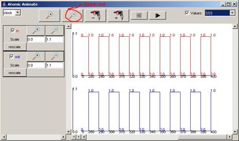
Figure 212: Formatted output
Select the model/component
to be visualized
1) The models/components available for visualization
can be seen in the drop-down list.
To select a model/component to be visualized, first
left-click on the drop-down list.
Note: The order of the models/components in the
drop-down list is arbitrary.
![]()
Figure 213: Selecting a model component
2) From the
drop-down list, select or left-click the model/component to be visualized. The
signals of the selected model/component will be displayed.
Note: For each
component, the order of the available signals (in the column below the
drop-down list) is arbitrary.
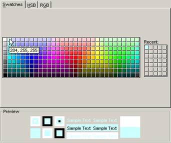
Also for each
component, the colors of the available signals are automatically assigned based
on their order. The first available signal will be red, the second blue, the
third green, etc.
The order of the visible visualization plots will correspond to the order of available signals that are selected for visualization.
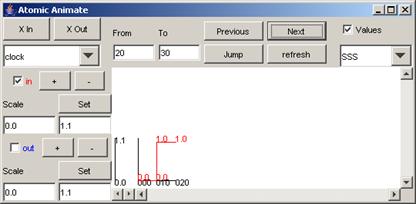
In this example, 4count is selected, and the signals
available are: q1 (green), q4 (brown), q3 (pinkn), and q2 (light blue). Since
all the available signals are checked, all the signals are plotted.
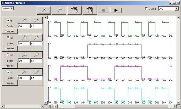
Figure 214: Viewing all signals
For the rest of the components in the drop-down list,
the available signals and range of output values for the entire simulation can
be seen in the following figures.
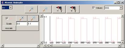
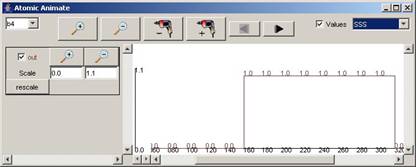
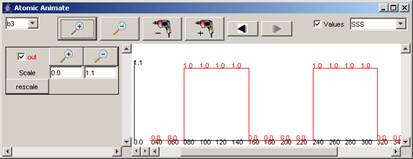
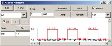
Figure 215: Available
signals and range of output values
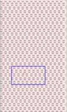
When the top
component is selected, the signals available are: in, clk, d1, d2, d3, d4, bo1,
bo2, bo3, bo4.
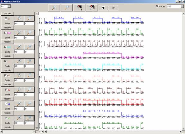
Figure 216: Viewing all signals in one window
Note: When the top component is selected, since the time
interval is initially set to correspond with the entire simulation, all the
available signals of the top component will be checked. Due to the number of
available signals in the top component, the space required to display the Scale
fields of the signals exceeds the height of the Atomic Animate visualization
window. The Scale fields can be made visible if the height of the visualization
window is increased.
It may not always
be possible to increase the height of the visualization window to accomodate
the Scale fields. (Please see Appendix B - 4BitCounter for more details.)
The visualization plots of the checked signals also
exceed the height of the Atomic Animate visualization window. The vertical scrollbar
can be used to view the visualization plots that are located beyond the bottom
edge of the window.
Availability of signals for
the selected model/component
A selected component can have multiple
signals (usually called ports).
When a component is selected, the signal
associated with the component can be selected to be displayed as a plot in the
visualization.
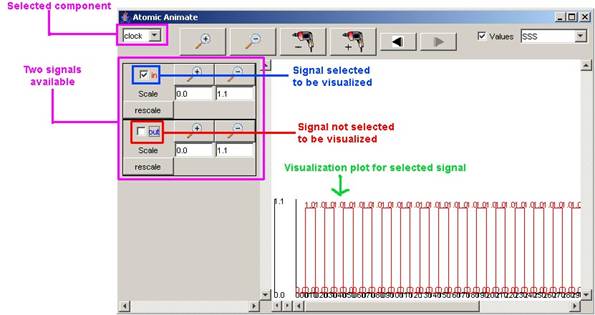
Figure 217: Selecting a signal to be displayed
A component will be displayed in the drop-down list if values are being sent to at least one signal of the component. (ie. if at least one signal is available for the component)
The following behaviour still applies: For a selected
component, the order of the available signals is arbitrary. The colours of the
available signals are automatically assigned based on their order. The first
available signal will be red, the second blue, the third green, etc. The order of the
visible visualization plots will correspond to the order of available signals
that are selected for visualization.
8.16.5 CoupledAnimate using: Coupled-DEVS
The message
values sent/received via ports within a coupled model can be visualized using
the graph (.gcm file) of the coupled model.
The visualization displays the output values with the corresponding
output ports, superimposed on the coupled model's graph.
The steps
required for visualizing the message values sent/received via the ports of a
coupled model are as follows:
1) In the Animate
menu, left-click on CoupledAnimate. A coupled animate dialog box will be
displayed.
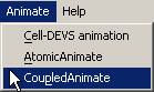
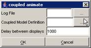
Figure 218:Choosing coupled animate
2) Specify the
Log file that contains the messages sent/received by the coupled-DEVS model to
be visualized (using the same procedure as for AtomicAnimate).
1)
Left-click on
the browse button for the Coupled Model Definition. A Set dialog will be
displayed. Select the .gcm file that corresponds to the coupled-DEVS model to
be visualized. After choosing the appropriate .gcm file, left-click on
Set.
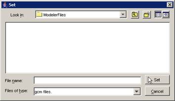
Figure 219: Set dialog box
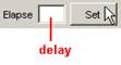
4) Type in the appropriate Delay between displays. The Delay value (milliseconds) will be
the amount of time the visualization waits between each update of the display.
(The speed of the visualization is determined by the Delay value.) By default,
the Delay is 1000 milliseconds (or 1 second).
If an invalid file type is chosen, the (blank)
visualization window will be displayed as follows:
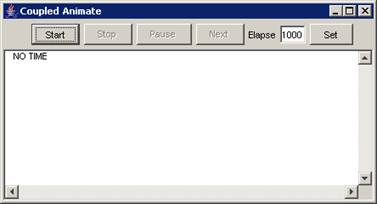
Figure 220: Blank view for invalid file type
The following example demonstrates the functionality of the Coupled Animate
visualization window, using the coupled model 4BitCounter.
8.16.6
CoupledAnimate
Example of Coupled-DEVS: 4BitCounter
To run this example, download the 4BitCounter project
from: http://www.angelfire.com/sc3/schao2/projects/4BitCounter.zip
4BitCounter is a coupled-DEVS model
composed of multiple atomic-DEVS models that each contain multiple output
signals.
In the Set and coupled animate dialogs,
open 4Counter.log and 4counter.gcm as the Log File and Coupled Model
Definition, respectively.
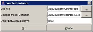
Figure 221: Opening the coupled model files
The coupled-DEVS model that sends/receives messages
within 4Counter.log, and that is represented in graphical form in 4counter.gcm,
will be available for visualization.
The following Coupled Animate visualization window
will be displayed.
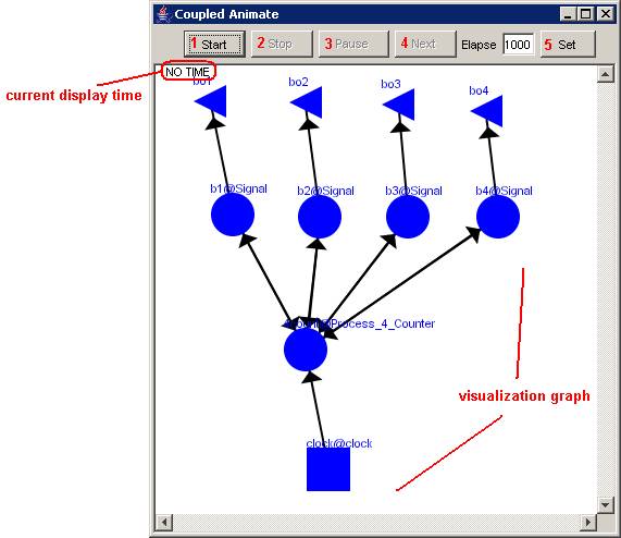
Figure 222: Coupled model visualization for 4bitcounter
The Coupled Animate visualization window has several
commands for the visualization, such as:
-start
the visualization (1)
-stop the
visualization (2)
-pause
the visualization (3)
-go to
the next display of the visualization (4)
-set the
delay between displays (5)
8.16.6.1
Start the visualization
1) Left-click the Start button. The visualization
will start and continue updating the graphical display, along with the
corresponding display time (according to the message times of the .log file).
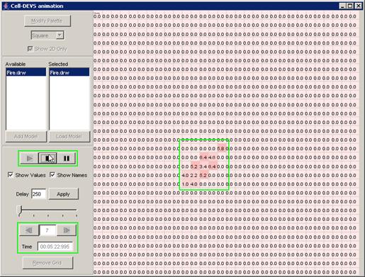
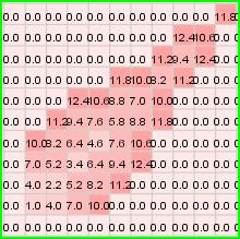
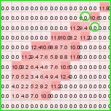
In this example, the visualization has been started,
and has the current display time of 00:00:00:070, with the output values
visible alongside their corresponding ports.
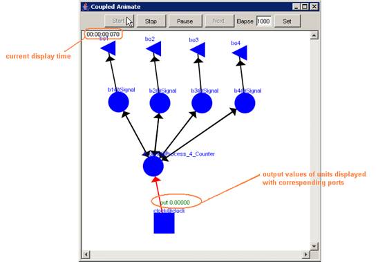
Figure 223: Viewing the current display time and output values of units
2) After the
visualization has started, it can be run to the end of the simulation time,
stopped, or paused.
- After the
visualization has started, if no other buttons are pressed, the visualization
will continue until it reaches the end of the simulation (ie. the last message
time in the .log file).
In this example,
after pressing the Start button, if no other buttons are pressed, the
visualization will continue until it reaches 00:00:00:400, which is when the
simulation ends in the .log file.
- The Stop and
Pause buttons are described in the following sections.
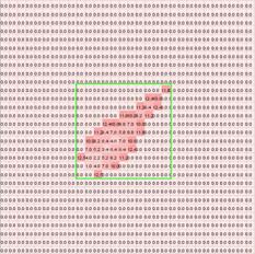
1) Left-click the Stop button. The visualization will
stop at the current display time. The output values occurring at the current
display time will remain visible on the graph.
In this example, the visualization has been stopped
at the current display time of 00:00:00:260, with the output values visible
alongside their corresponding ports.
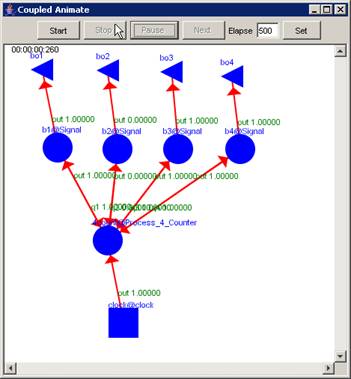
Figure 224: Stopped visualization
2) After the visualization has stopped, it can be
restarted (at the beginning of the simulation).
- After the visualization has stopped, if the Start
button is pressed, the visualization will restart only at the beginning of the
simulation, ie. at
- The Start button is described in the preceding
section.
8.16.6.3
Pause the visualization
1) Left-click the Pause button. The visualization
will pause at the current display time. The output values occurring at the
current display time will remain visible on the graph.
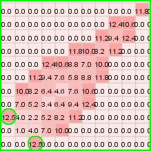
In this example, the Pause button is pressed after
the current display time of 00:00:00:380, pausing the visualization at
00:00:00:390, with the output values visible alongside their corresponding
ports.
![]()
![]()
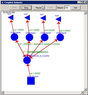
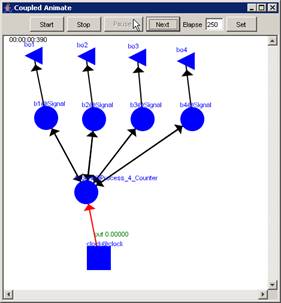
Figure 225: Pausing the visualization
2) After the visualization has paused, it can be
restarted (at the current display time), stopped, or incremented to the next
display.
- After the visualization has paused, if the Start
button is pressed, the visualization will restart at the current display time.
- The Start and Stop buttons are described in the
preceding sections. The Next button is described in the following section.
8.16.6.4
Go to the next display of the visualization
1) Left-click the
Next button. The visualization will increment to the next display, updating the
current display time and the output values visible on the graph.
This example
continues from the second graph in the previous section - 'Pause the
visualization'. In this example, with the visualization paused at 00:00:00:390,
the Next button has been pressed. The visualization is incremented to the next
display at 00:00:00:400, updating the current display time and the output
values displayed on the graph.
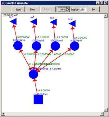
Figure 226: Resumed visualization
2) After the visualization has incremented to the
next display, it can be restarted (at the current display time), stopped, or
incremented again to the next display.
- After the visualization has incremented to the next
display, if the Start button is pressed, the visualization will restart at the
current display time.
- The Start and Stop buttons are described in the preceding
sections. The Next button is described in this section.
8.16.6.5
Set the delay between displays
1) Type the appropriate delay length (milliseconds)
in the Elapse field. Press Set.
The delay can be set while the
visualization is running (ie. after the visualization has been started), after
the visualization has been stopped, or while the visualization is paused (ie.
after the visualization has been paused).
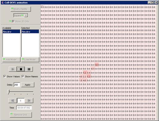
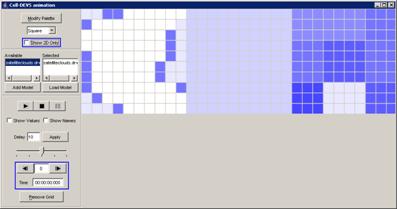
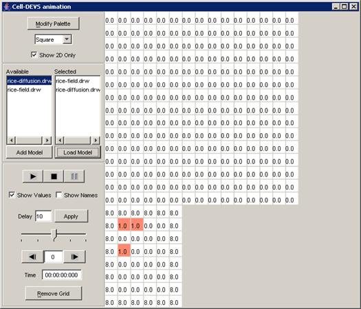
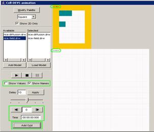
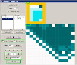
8.16.7 Cell-DEVS animation using: Atomic Cell-DEVS,
Coupled-DEVS
The steps required for visualizing the cell values of
an atomic cellular model are as follows:
1) In the Animate menu, left-click on Cell-DEVS
animation.
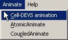
Figure 227: Cell-DEVS animation menu
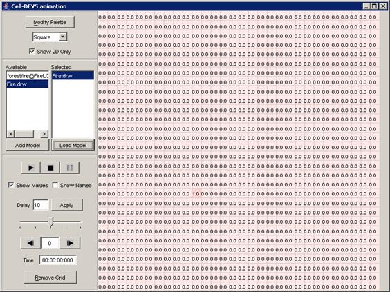
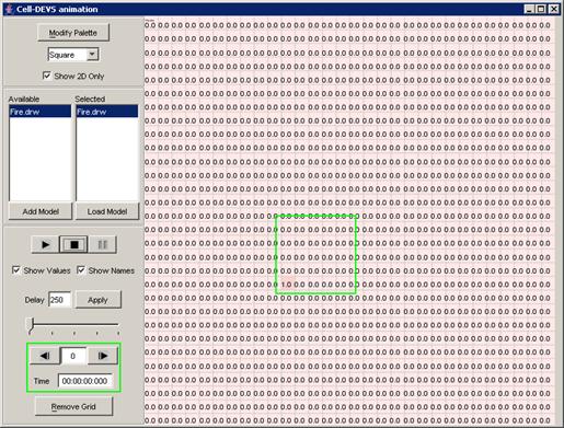
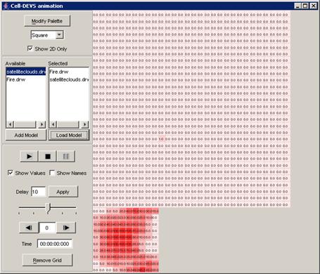
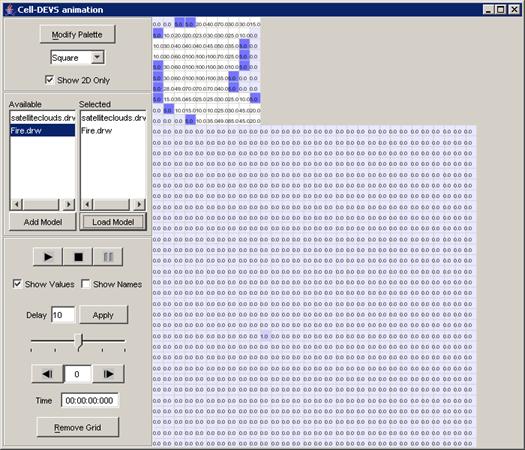
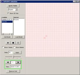
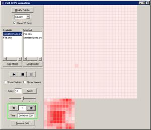
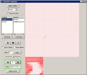
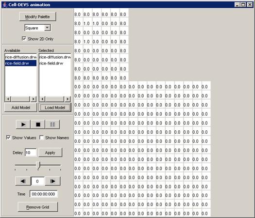
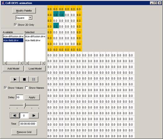
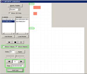
The following Cell-DEVS animation visualization
window will be displayed.
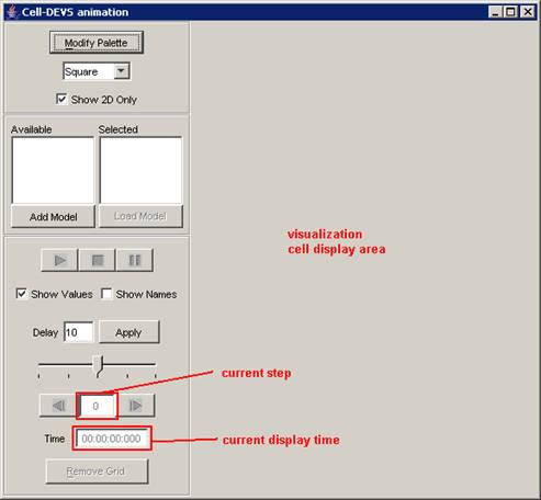
Figure 228: Cell-DEVS Animation window
2) A model must first be loaded before it can be
visualized. The loading of models will be described in upcoming sections.
3) The appearance of the visualization can be
modified before the visualization starts.
(The appearance of the visualization can also be modified while the
visualization is running.) The options
available for changing the appearance of the visualization will be described in
upcoming sections.
4) The individual steps/displays in the visualization
can be navigated to directly or indirectly. Navigating through the
visualization will be described in upcoming sections.
Thus, steps 2, 3, and 4 are the main steps for
visualizing an atomic Cell-DEVS model.
Each of the steps can be further broken down, as shown in the following
figure and list.
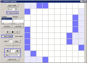
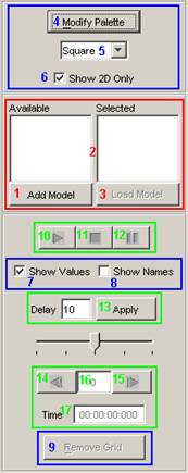 The Cell-DEVS animation visualization window has
functions that can be grouped according to the step in which the function is
involved. (See Figure
229)
The Cell-DEVS animation visualization window has
functions that can be grouped according to the step in which the function is
involved. (See Figure
229)
-loading models to be visualized
-modifying the appearance of the visualization
-running/navigating the visualization
For each of the main steps, there are several
functions.
For loading models to be visualized, functions
include:
-adding
models to be made available (1)
-selecting
available models to be loaded (2)
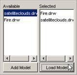
-loading
models to be visualized (3)
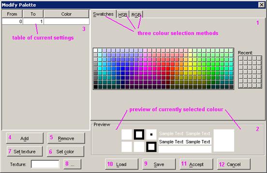
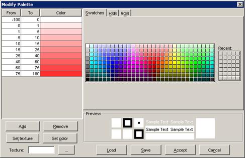
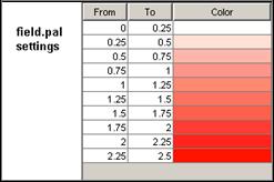
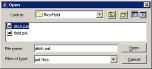
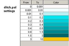
For modifying the appearance of the visualization,
functions include:
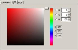
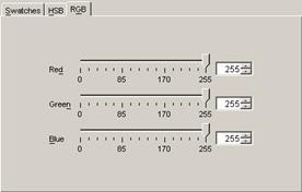
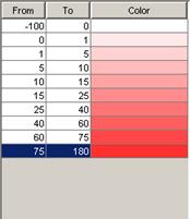
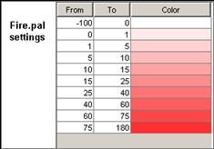
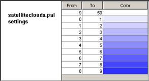
-modifying
the palette of the loaded models (4)
-selecting
the lattice type (5)
-toggle
between 2D and multidimensional display (6)
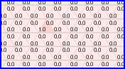
-showing
the cell values of the loaded models (7)
-showing
the names of the loaded models (8)
-toggle
the visibility of the grid of the lattice (9)
For running/navigating the visualization, functions
include:
-playing/starting
the visualization (10)
-stopping
the visualizaton (11)
-pausing
the visualization (12)
-set the
delay between steps of the visualization (13)
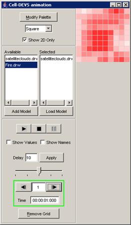
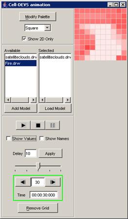
-go to
the previous/next step in the visualization (14,
15)
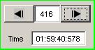
-go directly
to a particular step in the visualization (16)
-go
directly to a particular time in the visualization (17)
Figure 229: Options for
cell DEVS animation.
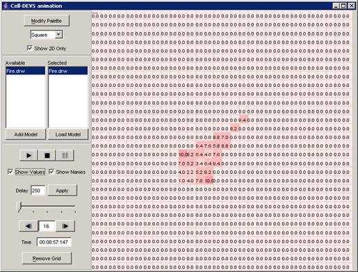
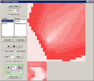
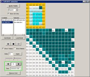
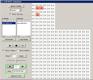
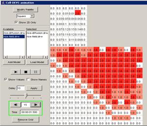
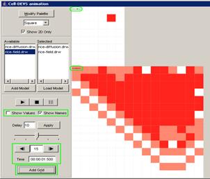
The following example demonstrates the functionality
of the Cell-DEVS animation visualization window, using the atomic Cell-DEVS
model Fire. Additional examples for a 3D atomic Cell-DEVS model
(SatelliteClouds) and a coupled-DEVS model (RiceField) follow.
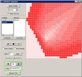
Cell-DEVS animation
Example of Atomic Cell-DEVS: Fire
To run this example, download the Fire project.
Fire is a 2D (two-dimensional) atomic
Cell-DEVS model.
8.16.8.1
Loading models to be visualized
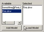
A model must first be loaded before it can be
visualized.
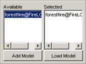
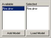
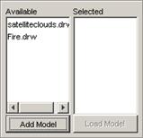
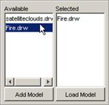
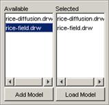
To load a model, the appropriate model must first be
added to the Available list. From the Available list, the appropriate model(s)
to be visualized must be selected (ie. to the Selected list). Once the models
to be visualized are in the Selected list, the models can then be loaded. These functions are described in the following
sections.
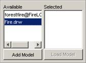
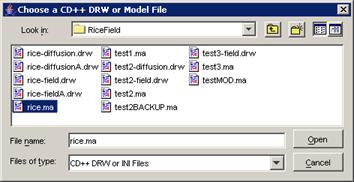
8.16.8.2
Adding models to the Available list
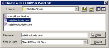
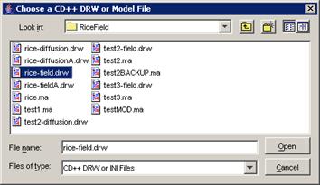
1) To add an atomic cellular model to the Available
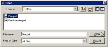
list, left-click the Add Model button. The Choose a CD++ DRW or Model File
dialog will be displayed.
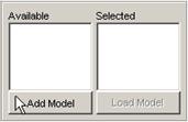
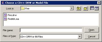
Figure 230: Adding an atomic cellular model
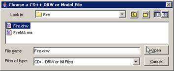
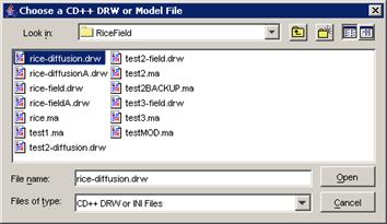
2) Two options are available: (a) choose a .ma file
and a .log file, or (b) choose only a .drw file.
(a) Choose the appropriate .ma file, and left-click
the Open button.
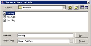
The Choose a CD++ LOG File dialog will be displayed.
Choose the appropriate .log file (corresponding
to the .ma file), and left-click the Open button.
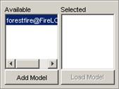
In this example, FireMA.ma is chosen in conjunction
with FireLOG.log.
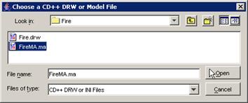
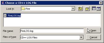
Figure 231: opening the Fire model
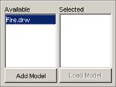
(b) Choose the appropriate .drw file, and left-click
the Open button.
In this example, Fire.drw is chosen.
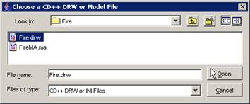
Figure 232: Choosing the appropriate drw file
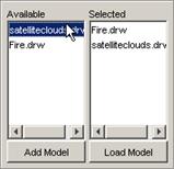
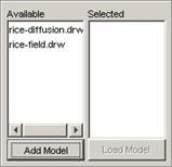
3) The atomic cellular model name will appear in the
Available list. The format of the model name (displayed in the Available list)
depends on the option chosen: